Two-layer synthetic causal simulation#
This tutorial demonstrates how to:
Load (or optionally generate) a synthetic two-layer dataset
Run CauTrigger in a known hierarchical setting (Layer 1 → Layer 2)
Visualize causal vs spurious latent spaces
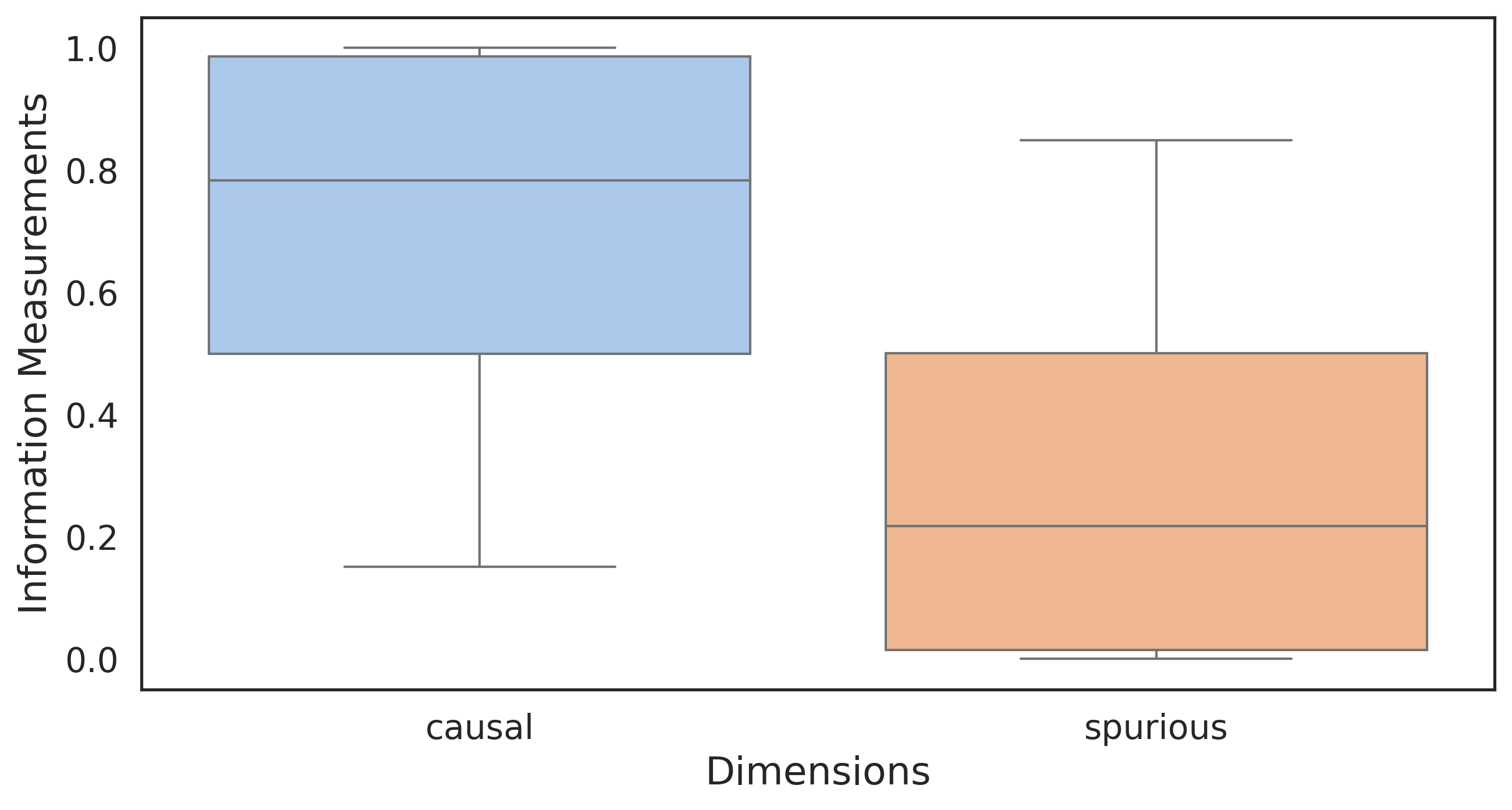
Examine information flow across layers
Global setup and imports#
import os
import sys
import math
import logging
import warnings
import numpy as np
import pandas as pd
import matplotlib.pyplot as plt
import seaborn as sns
import torch
import scanpy as sc
import gc

from scipy.stats import ttest_ind
from anndata import AnnData
from matplotlib.patches import Ellipse

from cautrigger.utils import set_seed
from cautrigger.model import CauTrigger2L, CauTrigger1L
from cautrigger.dataloaders import generate_two_layer_synthetic_data

sns.set_theme(style="white")
plt.rcParams.update({
    "font.size": 14,
    "axes.labelsize": 16,
    "axes.titlesize": 18,
    "xtick.labelsize": 14,
    "ytick.labelsize": 14,
    "legend.fontsize": 14,
    "figure.dpi": 300,
    "savefig.dpi": 300,
    "pdf.fonttype": 42,
    "ps.fonttype": 42,
})
warnings.filterwarnings("ignore")
logging.getLogger('matplotlib.font_manager').disabled = True

plt.rcParams['font.sans-serif'] = ['Arial']
plt.rcParams['font.family'] = 'sans-serif'
import os
import sys
import math
import logging
import warnings
import numpy as np
import pandas as pd
import matplotlib.pyplot as plt
import seaborn as sns
import torch
import scanpy as sc
import gc

from scipy.stats import ttest_ind
from anndata import AnnData
from matplotlib.patches import Ellipse

from cautrigger.utils import set_seed
from cautrigger.model import CauTrigger2L, CauTrigger1L
from cautrigger.dataloaders import generate_two_layer_synthetic_data

sns.set_theme(style="white")
plt.rcParams.update({
    "figure.figsize": (5, 3),
    "font.size": 14,
    "axes.labelsize": 16,
    "axes.titlesize": 18,
    "xtick.labelsize": 14,
    "ytick.labelsize": 14,
    "legend.fontsize": 14,
    "figure.dpi": 300,
    "savefig.dpi": 300,
    "pdf.fonttype": 42,
    "ps.fonttype": 42,
})
warnings.filterwarnings("ignore")
logging.getLogger('matplotlib.font_manager').disabled = True

plt.rcParams['font.sans-serif'] = ['Arial']
plt.rcParams['font.family'] = 'sans-serif'
plt.rcParams["figure.figsize"] = (5,3)
Paths and configuration#
# Root directories
base_dir = "../../02_simulation"
data_root = os.path.join(base_dir, "data")
out_root = os.path.join(base_dir, "output")

case_name = "2L_known_semi_hrc_hidden10_linear_cs40_p0.5_sc"
data_dir = os.path.join(data_root, case_name, 'dataset1')
output_dir = os.path.join(out_root, 'two_layer_known')

os.makedirs(output_dir, exist_ok=True)

np.random.seed(42)
set_seed(42)

adata_path = os.path.join(data_dir, "adata.h5ad")
Load (or optionally generate) synthetic dataset#
generate_data = False  # set True to regenerate

if generate_data:
    generation_args = dict(
        spurious_mode='semi_hrc',
        n_hidden=10,
        activation='linear',
        causal_strength=0.4,
        p_zero=0.5,
        simulate_single_cell=True,
    )
    adata = generate_two_layer_synthetic_data(seed=42, **generation_args)
else:
    adata = sc.read_h5ad(adata_path)

print(adata)
print(adata.var["layer"].value_counts())
AnnData object with n_obs × n_vars = 200 × 150
    obs: 'labels'
    var: 'feat_type', 'layer', 'is_causal'
    obsm: 'layer1', 'layer2'
layer
layer1    100
layer2     50
Name: count, dtype: int64
Train CauTrigger on layer 1#
layer1_vars = adata.var_names[adata.var["layer"] == "layer1"]
adata_step1 = sc.AnnData(
    X=adata.obsm["layer1"],
    obs=adata.obs.copy(),
    var=adata.var.loc[layer1_vars].copy()
)

model_1L = CauTrigger1L(
    adata_step1,
    n_causal=2,
    n_latent=10,
    n_layers_encoder=0,
    n_layers_decoder=0,
    n_layers_dpd=0,
    dropout_rate_encoder=0.0,
    dropout_rate_decoder=0.0,
    use_batch_norm='none',
    use_batch_norm_dpd=True,
    decoder_linear=False,
    dpd_linear=True,
    init_thresh=0.4,
)

model_1L.train(max_epochs=200, stage_training=True, weight_scheme="sim")
df_step1, _ = model_1L.get_up_feature_weights(method='SHAP', normalize=False, sort_by_weight=True)
model_1L.compute_information_flow(save_fig=True, skip_single_info=True, save_dir=output_dir)
(            0         1         2         3         4         5         6  \
 0    0.523847  0.006137  0.004729  0.000408  0.000170  0.182491  0.245564
 1    0.740391  0.003828  0.005954  0.000753  0.000075  0.066525  0.156985
 2    0.710571  0.009342  0.003520  0.000502  0.000051  0.073055  0.179951
 3    0.798089  0.003373  0.002880  0.000330  0.000043  0.035886  0.145742
 4    0.932918  0.000389  0.000574  0.000045  0.000014  0.016412  0.045849
 ..        ...       ...       ...       ...       ...       ...       ...
 195  0.981886  0.002246  0.000405  0.000099  0.000111  0.005186  0.007248
 196  0.710309  0.009786  0.005422  0.001209  0.000264  0.068652  0.138121
 197  0.920478  0.002920  0.001324  0.000187  0.000067  0.026001  0.037630
 198  0.661235  0.017686  0.010498  0.001150  0.000336  0.088575  0.186522
 199  0.214908  0.055392  0.018668  0.004176  0.001534  0.258732  0.322838

             7         8         9
 0    0.025873  0.010042  0.000740
 1    0.020035  0.005039  0.000415
 2    0.017433  0.005236  0.000340
 3    0.007716  0.005637  0.000304
 4    0.003154  0.000573  0.000072
 ..        ...       ...       ...
 195  0.002211  0.000505  0.000103
 196  0.058316  0.007061  0.000859
 197  0.008139  0.002922  0.000332
 198  0.021504  0.011639  0.000855
 199  0.091444  0.026984  0.005323

 [200 rows x 10 columns],
        causal  spurious
 0    0.241761  0.758239
 1    0.281648  0.718352
 2    0.253769  0.746231
 3    0.610673  0.389327
 4    0.345402  0.654598
 ..        ...       ...
 195  0.987337  0.012663
 196  0.511487  0.488513
 197  0.814984  0.185016
 198  0.575370  0.424630
 199  0.564169  0.435831

 [200 rows x 2 columns])
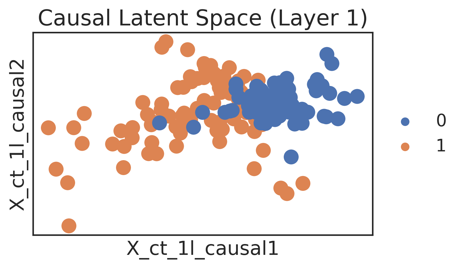
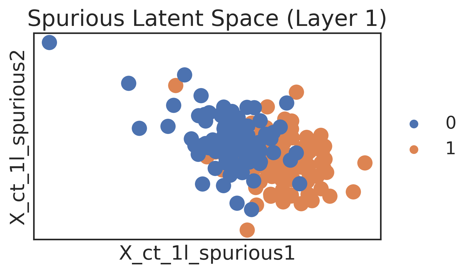
Layer 1 latent space visualization#
adata_step1.obsm['X_ct_1l_causal'] = model_1L.get_model_output()['latent'][:, :2]
adata_step1.obsm['X_ct_1l_spurious'] = model_1L.get_model_output()['latent'][:, -2:]
adata_step1.obs.labels = adata_step1.obs['labels'].astype(str)

sc.pl.embedding(
    adata_step1, basis='X_ct_1l_causal', color='labels',
    title='Causal Latent Space (Layer 1)', show=True
)

sc.pl.embedding(
    adata_step1, basis='X_ct_1l_spurious', color='labels',
    title='Spurious Latent Space (Layer 1)', show=True
)
Train CauTrigger on layer 2 and layer1#
topk = 20
layer2_vars = adata.var_names[adata.var["layer"] == "layer2"]
df_layer1 = df_step1.loc[layer1_vars]
topk_indices = df_layer1["weight"].values.argsort()[-topk:]
X_down = adata.obsm["layer1"][:, topk_indices]

adata_step2 = sc.AnnData(
    X=adata.obsm["layer2"],
    obs=adata.obs.copy(),
    var=adata.var.loc[layer2_vars].copy(),
    obsm={"X_down": X_down}
)

model_2L = CauTrigger2L(
    adata_step2,
    n_causal=2,
    n_latent=10,
    n_layers_encoder=0,
    n_layers_decoder=0,
    n_layers_dpd=0,
    dropout_rate_encoder=0.0,
    dropout_rate_decoder=0.0,
    use_batch_norm='none',
    use_batch_norm_dpd=True,
    decoder_linear=False,
    dpd_linear=True,
    init_thresh=0.4,
)

model_2L.train(max_epochs=200, stage_training=True, weight_scheme="sim")
df_step2, _ = model_2L.get_up_feature_weights(method='SHAP', normalize=False, sort_by_weight=True)
df_step2 = df_step2.loc[layer2_vars]

model_2L.compute_information_flow(save_fig=True, skip_single_info=True, save_dir=output_dir)
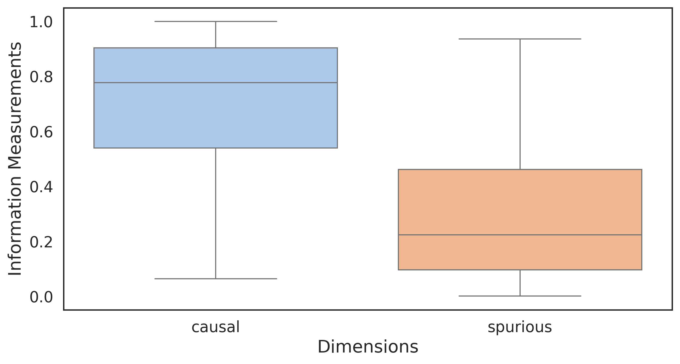
(            0         1         2         3         4         5         6  \
 0    0.490880  0.307667  0.006788  0.046713  0.023150  0.060010  0.022715
 1    0.271371  0.586589  0.007083  0.017069  0.006886  0.033169  0.005213
 2    0.137355  0.726735  0.024560  0.035258  0.008943  0.002612  0.000808
 3    0.693573  0.164123  0.004589  0.026349  0.009502  0.056385  0.006379
 4    0.119563  0.658189  0.025053  0.095344  0.005562  0.004343  0.000766
 ..        ...       ...       ...       ...       ...       ...       ...
 195  0.468126  0.010783  0.074487  0.035272  0.084719  0.160081  0.013601
 196  0.219003  0.099201  0.127269  0.014876  0.122657  0.202516  0.003111
 197  0.302682  0.052102  0.057741  0.045482  0.111329  0.196043  0.032698
 198  0.481469  0.041554  0.067413  0.054515  0.068185  0.137188  0.023968
 199  0.286295  0.348240  0.005486  0.017031  0.049375  0.113826  0.013567

             7         8         9
 0    0.004838  0.027188  0.010050
 1    0.013064  0.041950  0.017606
 2    0.022554  0.009248  0.031926
 3    0.014615  0.019241  0.005244
 4    0.009597  0.039863  0.041719
 ..        ...       ...       ...
 195  0.043754  0.021860  0.087316
 196  0.004415  0.124984  0.081967
 197  0.060972  0.056317  0.084632
 198  0.047068  0.019811  0.058826
 199  0.007329  0.094901  0.063950

 [200 rows x 10 columns],
        causal  spurious
 0    0.727863  0.272136
 1    0.885933  0.114067
 2    0.870725  0.129275
 3    0.895511  0.104489
 4    0.925025  0.074975
 ..        ...       ...
 195  0.481558  0.518441
 196  0.616598  0.383401
 197  0.303379  0.696621
 198  0.522915  0.477084
 199  0.797973  0.202027

 [200 rows x 2 columns])
Layer 2 latent space visualization#
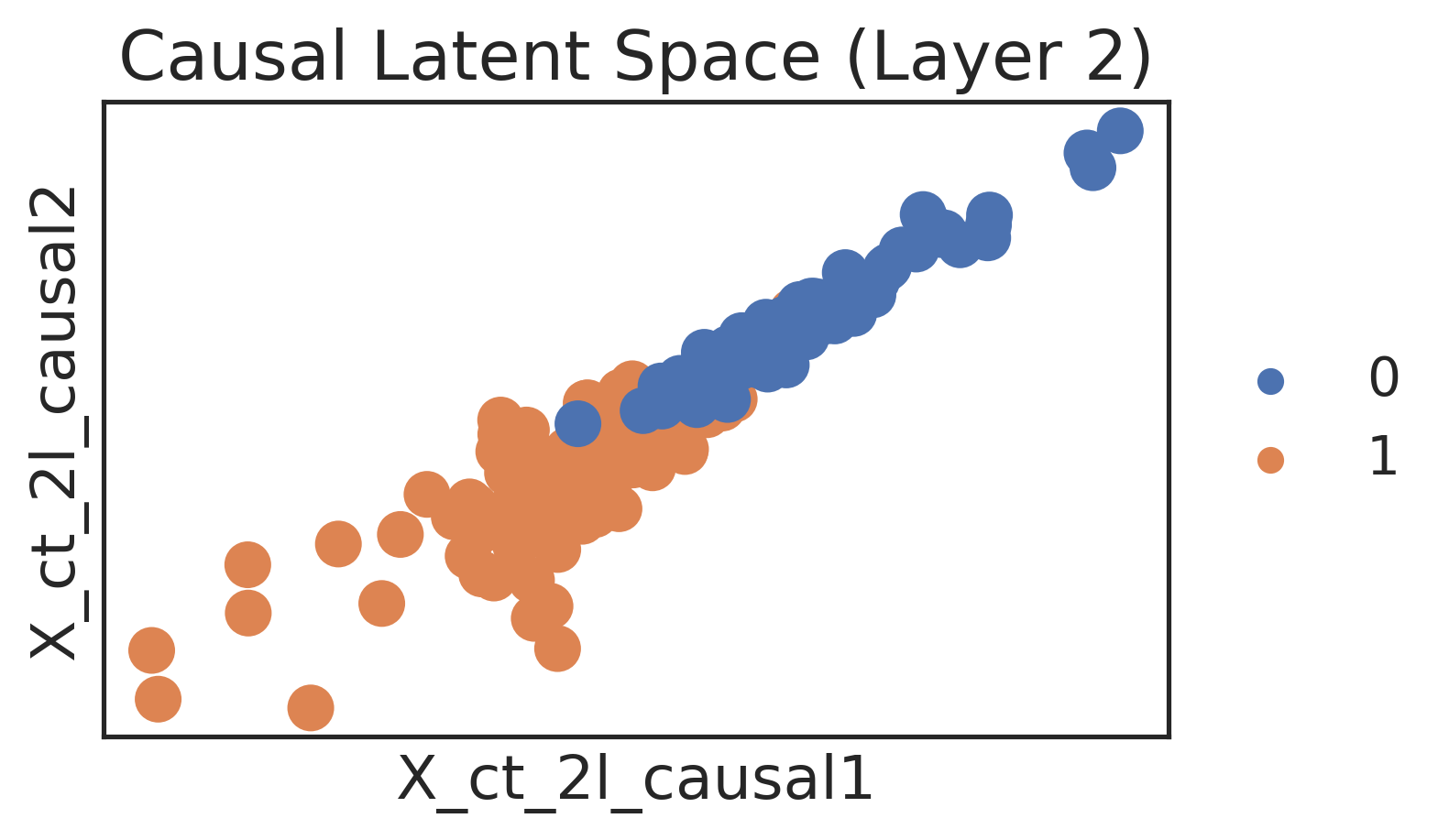
adata_step2.obsm['X_ct_2l_causal'] = model_2L.get_model_output()['latent'][:, :2]
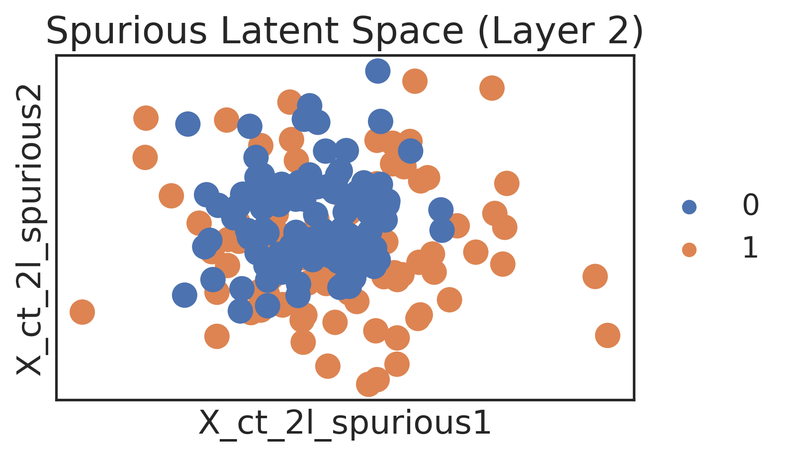
adata_step2.obsm['X_ct_2l_spurious'] = model_2L.get_model_output()['latent'][:, -2:]
adata_step2.obs.labels = adata_step2.obs['labels'].astype(str)

sc.pl.embedding(
    adata_step2, basis='X_ct_2l_causal', color='labels',
    title='Causal Latent Space (Layer 2)', show=True
)

sc.pl.embedding(
    adata_step2, basis='X_ct_2l_spurious', color='labels',
    title='Spurious Latent Space (Layer 2)', show=True
)
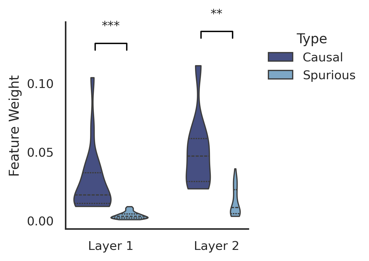
Causal vs. spurious weights across layers#
# Build tidy DataFrame
df = pd.DataFrame({
    'weight': np.concatenate([df_step1['weight'].values, df_step2['weight'].values]),
    'type':   ['Causal'] * 20 + ['Spurious'] * 80 + ['Causal'] * 10 + ['Spurious'] * 40,
    'layer':  ['Layer 1'] * (20 + 80) + ['Layer 2'] * (10 + 40),
})

# Color palette (publication-friendly)
type_palette = {
    'Causal':   '#3E4A89',
    'Spurious': '#74A9CF'
}

plt.figure(figsize=(4.5, 3.2))  # smaller and website-friendly
ax = sns.violinplot(
    data=df,
    x="layer",
    y="weight",
    hue="type",
    palette=type_palette,
    inner="quartile",
    cut=0,
    bw=0.4,
    width=0.7,
    linewidth=1.0,
    dodge=True,
    saturation=0.80,
)

# ========== significance annotation ==========
from scipy.stats import ttest_ind

layers = df['layer'].unique()
x_offsets = {'Causal': -0.15, 'Spurious': 0.15}

for i, layer in enumerate(layers):
    subset = df[df['layer'] == layer]

    causal_vals   = subset[subset['type'] == 'Causal']['weight']
    spurious_vals = subset[subset['type'] == 'Spurious']['weight']

    _, pval = ttest_ind(causal_vals, spurious_vals, equal_var=False)

    if pval < 0.0001:
        sig = '****'
    elif pval < 0.001:
        sig = '***'
    elif pval < 0.01:
        sig = '**'
    elif pval < 0.05:
        sig = '*'
    else:
        sig = 'ns'

    x1 = i + x_offsets['Causal']
    x2 = i + x_offsets['Spurious']
    y  = max(causal_vals.max(), spurious_vals.max()) + 0.025

    ax.plot([x1, x1, x2, x2],
            [y-0.005, y, y, y-0.005],
            c='black', lw=1.1)

    ax.text((x1 + x2)/2, y + 0.008, sig,
            ha='center', va='bottom', fontsize=10)

# axis beautify
plt.xlabel("")
plt.ylabel("Feature Weight", fontsize=11)
plt.xticks(fontsize=10)
plt.yticks(fontsize=10)
plt.legend(title='Type',
           fontsize=10, title_fontsize=11,
           frameon=False,
           loc='upper left',
           bbox_to_anchor=(1.05, 1.0))

sns.despine()
plt.tight_layout()
plt.show()